New year, new post. Here I am again with a new topic that I found interesting to read after watching the videos of 3Blue1Brown on deep learning. It seems like the “Hello world!” of machine learning is making a neural network that recognizes handwritten digits, so today’s post will be about that.
The multilayer perceptron
An MLP (Multilayer perceptron) is a network of “neurons” connected in a forward manner from input neurons to the outputs.
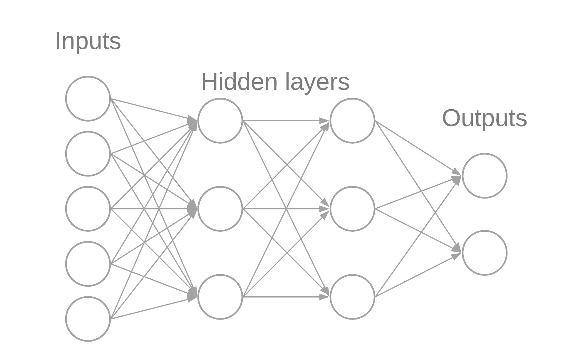
The value of the neurons on each layer after the input is just a weighted sum of the values of the previous neurons passed through an activation function plus a bias. In this case for a perceptron:
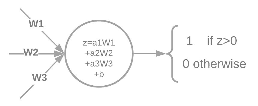
The term “MLP” seems to be used to generalize any neural network that not necessarily uses that activation function. Later I’ll show an interesting activation function that’s pretty similar to this one of a perceptron
Feedfowarding to the outputs
The beauty of this topic is that everything is basically linear algebra and calculus. If we represent every weight, bias, and the value of a neuron per layer using a matrix, then we can use simple matrix operations to work our way to the outputs. For this, I’ll use the superscript as the layer and the subscript as the output \(a\) of the neuron and bias \(b\)
\[\begin{bmatrix} a^0_1 \\ a^0_2 \\ a^0_3 \\ a^0_4 \\ a^0_5 \end{bmatrix} \space\begin{bmatrix} a^1_1 \\ a^1_2 \\ a^1_3 \end{bmatrix} \space\begin{bmatrix} a^2_1 \\ a^2_2 \\ a^2_3 \end{bmatrix} \space\begin{bmatrix} a^3_1 \\ a^3_2 \end{bmatrix}\] \[\begin{bmatrix} b^1_1 \\ b^1_2 \\ b^1_3 \end{bmatrix} \space\begin{bmatrix} b^2_1 \\ b^2_2 \\ b^2_3 \end{bmatrix} \space\begin{bmatrix} b^3_1 \\ b^3_2 \end{bmatrix}\]For the weights, the superscript will indicate to which layer they are connecting, and the subscript will show the connection of the neuron n to the neuron m of the previous layer
\[\begin{bmatrix} w^1_{11} & w^1_{12} & w^1_{13} & w^1_{14} & w^1_{15} \\ w^1_{21} & w^1_{22} & w^1_{23} & w^1_{24} & w^1_{25} \\ w^1_{31} & w^1_{32} & w^1_{33} & w^1_{34} & w^1_{35} \end{bmatrix} \space \begin{bmatrix} w^2_{11} &w^2_{12} &w^2_{13} \\ w^2_{21} &w^2_{22} &w^2_{23} \\ w^2_{31} &w^2_{32} &w^2_{33} \end{bmatrix} \space \begin{bmatrix} w^2{11} & w^2{12} & w^2{13} \\ w^2{21}& w^2{22} &w^2{23} \end{bmatrix}\]Given the rules of matrix multiplication, for example, we multiply the inputs by the weights that connect to the next layer then we will get a matrix of size 3x1, the same number of neurons of our next layer.
\[\begin{bmatrix} w^1_{11} & w^1_{12} & w^1_{13} & w^1_{14} & w^1_{15} \\ w^1_{21} & w^1_{22} & w^1_{23} & w^1_{24} & w^1_{25} \\ w^1_{31} & w^1_{32} & w^1_{33} & w^1_{34} & w^1_{35} \end{bmatrix} \begin{bmatrix} a^0_1 \\ a^0_2 \\ a^0_3 \\ a^0_4 \\ a^0_5 \end{bmatrix}=\begin{bmatrix} a^0_1w^1_{11} + a^0_2w^1_{12} + a^0_3w^1_{13} + a^0_4w^1_{14} + a^0_5w^1_{15} \\ a^0_1w^1_{21} + a^0_2w^1_{12} + a^0_3w^1_{23} + a^0_4w^1_{24} + a^0_5w^1_{25} \\ a^0_1w^1_{31} + a^0_2w^1_{32} + a^0_3w^1_{33} + a^0_4w^1_{34} + a^0_5w^1_{35} \end{bmatrix}\]Then adding the bias and applying our activation function \(f\) element-wise to the resulting vector will give us the value of the neurons for our first hidden layer.
\[f\left( \begin{bmatrix} a^0_1w^1_{11} + a^0_2w^1_{12} + a^0_3w^1_{13} + a^0_4w^1_{14} + a^0_5w^1_{15} \\ a^0_1w^1_{21} + a^0_2w^1_{12} + a^0_3w^1_{23} + a^0_4w^1_{24} + a^0_5w^1_{25} \\ a^0_1w^1_{31} + a^0_2w^1_{32} + a^0_3w^1_{33} + a^0_4w^1_{34} + a^0_5w^1_{35} \end{bmatrix}+\begin{bmatrix} b^1_1 \\ b^1_2 \\ b^1_3 \end{bmatrix} \right)=\begin{bmatrix} a^1_1 \\ a^1_2 \\ a^1_3 \end{bmatrix}\]Doing this all the way to the outputs will give you the prediction of the network with its current weights and biases. It could be right, or it could be wrong.
Deep learning (with backpropagation)
Deep learning is a set of rules defining how our network will “learn” to give the best possible output. We can see our network as a function that takes X inputs, N biases and M weights, process them and gives out an output vector. In order to train it, we need to have a large set of data that will have a series of inputs and the expected output, from here finding how far the predictions are from the expected outputs will allow us to tune the weights and biases until we start getting the predictions we want. Backpropagation does this by finding how much each parameter of the network affects the value of some cost function and reducing it. For this example our cost function will be:
\[C_o=\frac{1}{2}\sum_{i}^{n}(y_i-a_i)^2\]By using calculus we can create a gradient of our function that will allow us to tune each weight and bias in order to get each output \(a_i\) closer to those expected \(y_i\) outputs. Let’s see how is done for the weights and biases that go from the first neuron of the second-last layer to the first neuron of our last layer:
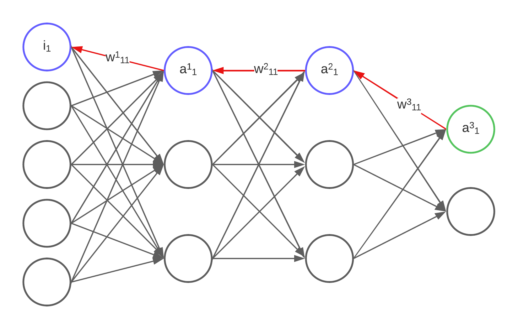
Using the multivariable chain rule will allow us to find how much one bias and weight affects the cost
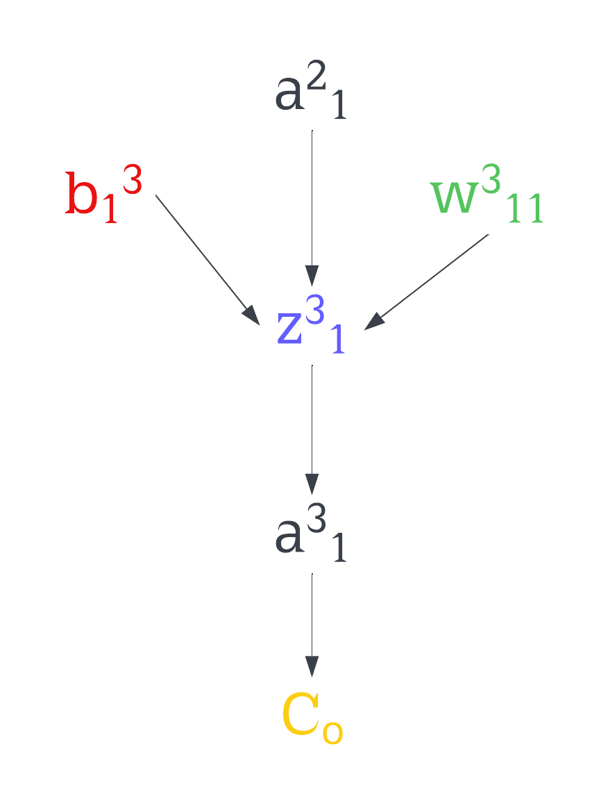
Let’s say we want to find how much that bias affects the cost. This can done by computing the derivative of the cost with respect to the bias.
\[\frac{\partial C_o}{\partial b^3_1}\]The chain rule tells us that this derivative will be equal to the products of all those derivatives with respect to the element that follows them from bottom to top
\[\frac{\partial C_o}{\partial b^3_1}=\frac{\partial C_o}{\partial a^3_1}\cdot\frac{\partial a^3_1}{\partial z^3_1}\cdot \frac{\partial z^3_1}{\partial b^3_1}\]We know that
\[\begin{matrix} C_o=\frac{1}{2}[(y_1-a^3_1)^2+(y_2-a^3_2)^2]\\ z^3_1=(a^2_1w^3_{11}+a^2_2w^3_{12}+a^2_3w^3_{13})+b^3_1\\ a^3_1=f(z^3_1) \end{matrix}\]So the derivatives of those functions with respect to what’s needed end up being:
\[\begin{matrix} \frac{\partial C_o}{\partial a^3_1}=(y_1-a^3_1),\space \frac{\partial a^3_1}{\partial z^3_1}=f'(z^3_1),\space \frac{\partial z^3_1}{\partial b^3_1}=1 \\ \Rightarrow \frac{\partial C_o}{\partial b^3_1}=(y_1-a^3_1)f'(z^3_1) \end{matrix}\]We do this for the rest of functions at the top of the chain
\[\begin{matrix} \frac{\partial C_o}{\partial w^3_{11}}=\frac{\partial C_o}{\partial a^3_1}\cdot\frac{\partial a^3_1}{\partial z^3_1}\cdot \frac{\partial z^3_1}{\partial w^3_{11}}=\frac{\partial C_o}{\partial b^3_1}\cdot\frac{\partial z^3_1}{\partial w^3_{11}} \\ \frac{\partial C_o}{\partial a^2_{1}}=\frac{\partial C_o}{\partial a^3_1}\cdot\frac{\partial a^3_1}{\partial z^3_1}\cdot \frac{\partial z^3_1}{\partial a^2_{1}}=\frac{\partial C_o}{\partial b^3_1}\cdot\frac{\partial z^3_1}{\partial a^2_{1}} \\ \Rightarrow \frac{\partial z^3_1}{\partial w^3_{11}}=a^2_1,\space \frac{\partial z^3_1}{\partial a^3_{2}}=w^3_{11} \\ \Rightarrow \frac{\partial C_o}{\partial w^3_{11}}=a^2_1(y_1-a^3_1)f'(z^3_1), \space \frac{\partial C_o}{\partial a^2_{1}}=w^3_{11}(y_1-a^3_1)f'(z^3_1) \end{matrix}\]And just like this, work your way up to the inputs with each neuron, bias and weight
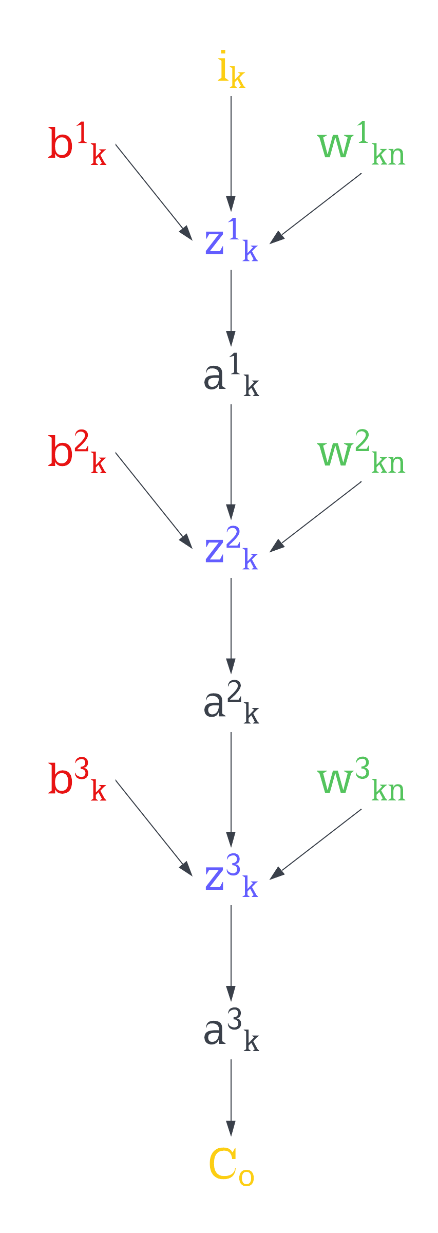
Since a network will usually deal with a lot of possible results, we need to average these derivatives over all training samples and only then, subtract to the weight or bias that averaged derivative multiplied by some factor \(\gamma\)
\[\begin{matrix} b^L_k=b^L_k-\gamma \cdot \frac{1}{s}\sum_{}^{s} \frac{\partial C_o}{\partial b^L_k}\\ w^L_{kn}=w^L_{kn}-\gamma \cdot \frac{1}{s}\sum_{}^{s} \frac{\partial C_o}{\partial w^L_{kn}} \end{matrix}\]Computing with matrices
Once again, these operations for all weights and biases can be done “all at once” per layer using matrices, allowing us to use libraries optimized for matrix operations and linear algebra. So now we will make matrices/vectors to do these layer operations. As you have seen, to compute the derivative of weight and previous neuron, multiply the derivative of the bias by the value of the previous neuron or weight, this way we create a new vector \(\delta^l\) that will be composed of the bias derivatives of each neuron in the layer \(l\)
\[\delta^3=\begin{bmatrix} b^3_1 \\ b^3_2 \end{bmatrix}\]To compute this \(\delta^3\) we do the same thing as if it were a single bias, with the difference that we’ll be doing element-wise operations with vectors/matrices.
\[\begin{matrix} \Delta C_o=\begin{bmatrix} y_1-a^3_1 \\ y_2-a^3_2 \end{bmatrix}=y-a^3, \space z^3=\begin{bmatrix} w^3_{11}a^2_1+w^3_{12}a^2_2 \\ w^3_{21}a^2_1+w^3_{21}a^2_2 \end{bmatrix}+\begin{bmatrix} b^3_1 \\ b^3_2 \end{bmatrix}=w^3a^2+b^3 \\ \Rightarrow \delta³=\Delta C_o\odot f'(z^3) \\ \odot \space is\space elementwise\space multiplication \end{matrix}\]From here we compute \(\Delta w^3\) and \(\delta^2\) for it to be used on the previous layer
\[\begin{matrix} \Delta w^3=\delta^3(a^2)^T \\ \delta^2=(w^3)^T\delta^3 \odot f'(z^2) \end{matrix}\]And we work our way to the inputs
\[\begin{matrix} \Delta w^2=\delta^3(a^1)^T\\ \delta^1=(w^2)^T\delta^2 \odot f'(z^1)\\ \Delta w^1=\delta^1i^T \end{matrix}\]Then (after averaging those vectors) we subtract by our deltas many times as necessary to bring the loss to a minimum
\[\begin{matrix} b^1 = b^1-\gamma\delta^1 \\ w^1 = w^1-\gamma\Delta w^1 \\ b^2 = b^2-\gamma\delta^2 \\ w^2 = w^2-\gamma\Delta w^2 \\ b^3 = b^3-\gamma\delta^3 \\ w^3 = w^3-\gamma\Delta w^3 \end{matrix}\]It’s very important to note that since we initialize the weights and biases with random values it’s possible that we won’t find the global minima of the loss.
Handwritten number recognition
The apparent “Hello world!” of machine learning. The idea is to take a 28x28 image of some written number and make a network that can classify the number from 0 to 9
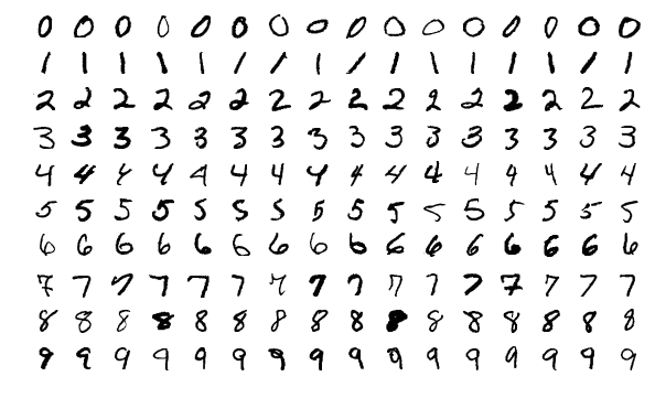
This network will have four layers: 784 inputs (flattened 28x28 image matrix), two 16 neuron hidden layers, and 10 neurons output.
The activation function for the hidden layers will be the \(ReLU\). This function and its derivative are easy to compute:
\[\begin{matrix} ReLU(x)=\left\{ \begin{array}{cl} x & : \ x \geq 0 \\ 0 & : \ x < 0 \end{array} \right. \\ ReLU'(x)=\left\{ \begin{array}{cl} 1 & : \ x \geq 0 \\ 0 & : \ x < 0 \end{array} \right. \end{matrix}\]Since this is a classifier I’ll be using the softmax function at the outputs, this will turn the values of the output to a way that everything adds to 1, so each value of the output is a probability of the image being that number
\[\sigma(\overrightarrow{z})_i = \frac{e^{z_i}}{\sum^{K}_{j}e^{z_j}}\]The derivative of this function is quite interesting to compute, to make it easier let’s start by computing the derivative of the first element in a 2x1 matrix
\[\begin{matrix} z=\begin{bmatrix} v_1 \\ v_2 \end{bmatrix},\space \sigma(z)_1=\frac{e^{v_1}}{e^{v_1}+e^{v_2}} \\ \frac{d}{dx}\frac{f}{g}=\frac{f'g-g'f}{g^2}\Rightarrow \frac{\partial \sigma(z)_1}{v_1}=\frac{e^{v_1}(e^{v_1}+e^{v_2})-e^{2v_1}}{(e^{v_1}+e^{v_2})^2} \\ =\frac{e^{v_1}}{e^{v_1}+e^{v_2}}-\frac{e^{2v_1}}{(e^{v_1}+e^{v_2})^2}=\sigma(z)_1-\sigma^2(z)_1 \end{matrix}\]Try doing this for more elements, and you’ll find that:
\[\frac{\partial\sigma(\overrightarrow{z})_i}{\partial z_i}=\sigma(\overrightarrow{z})_i-\sigma^2(\overrightarrow{z})_i=\sigma(\overrightarrow{z})_i(1-\sigma(\overrightarrow{z})_i)\]Then for the cost function I’ll be using Cross-entropy loss:
\[C_o(a)=-\sum^{}_{i}y_iln(a_i)\]Using this function as the cost function will give us a short expression for \(\delta^4\). To explain this I’ll go back to a network that has two outputs
\[a=\begin{bmatrix} a_1 \\ a_2 \end{bmatrix},\space y=\begin{bmatrix} y_1 \\ y_2 \end{bmatrix},\space C_o(a)=-y_1ln(a_1)-y_2ln(a_2)\]We know that for the ouputs \(\delta=\Delta C_o\odot f'(z)\), so we compute:
\[\Delta C_o=\begin{bmatrix} -\frac{y_1}{a_1} \\ -\frac{y_2}{a_2} \end{bmatrix},\space \delta=\begin{bmatrix} y_1a_1-y_1 \\ y_2a_2-y_2 \end{bmatrix}=y\odot\begin{bmatrix} a_1-y_1 \\ a_2-y_2 \end{bmatrix}\]I don’t know the best way to explain this, but by abusing the fact that this is a classification problem \(y\) will always be a matrix where only one element is equal to 1 and the rest are zeros, the sum is always one so we can simplify \(\delta\) to (a more detailed explanation here):
\[\delta=a-y\]Implementation
Once again I’ll be using GNU Octave because libBLAS is a thing and there’s no need to reinvent the wheel. I got the training and test dataset from here.
old_state = warning ("off", "Octave:shadowed-function");
pkg load statistics
pkg load io
warning (old_state);

%A_1=[784 1]
global A_2=double(unifrnd(0,1,[16 1]));
global A_3=double(unifrnd(0,1,[16 1]));
global A_4=double(unifrnd(0,1,[10 1]));


global W_12 = double(unifrnd(0,1,[16 784]));
global B_2  = double(unifrnd(0,1,[16 1]));

global W_23 = double(unifrnd(0,1,[16 16]));
global B_3  = double(unifrnd(0,1,[16 1]));

global W_34 = double(unifrnd(0,1,[10 16]));
global B_4  = double(unifrnd(0,1,[10 1]));

%Activations
function y = relu(x)
    y = max(0, x);
end

function y = relu_derivative(x)
    y = (x > 0);
end

function y = softmax(x)
    s=x-max(x);
    y = exp(s) ./ sum(exp(s));
end

%Backpropagation
function [d_bias_4,d_weight_4, d_bias_3,d_weight_3, d_bias_2,d_weight_2]=backpropagate(inputs,outputs)
    global A_2;
    global A_3;
    global A_4;
    global W_12;
    global B_2;
    global W_23;
    global B_3;
    global W_34;
    global B_4;

    z_2=(W_12*inputs)+B_2;
    A_2=relu(z_2);

    z_3=(W_23*A_2)+B_3;
    A_3=relu(z_3);

    z_4=(W_34*A_3)+B_4;
    A_4=softmax(z_4);

    %1 / size(inputs, 2) is just to scale the gradient
    d_cost = A_4 - outputs;
    d_weight_4 = (1 / size(inputs, 2)) * d_cost * A_3';
    d_bias_4 = (1 / size(inputs, 2))*d_cost;

    d_cost = (W_34' * d_cost) .* relu_derivative(z_3);
    d_weight_3 = (1 / size(inputs, 2))*d_cost * A_2';
    d_bias_3 = (1 / size(inputs, 2))*d_cost;

    d_cost = (W_23' * d_cost) .* relu_derivative(z_2);
    d_weight_2 = (1 / size(inputs, 2))*d_cost * inputs';
    d_bias_2 = (1 / size(inputs, 2))*d_cost;

endfunction

function [d_b4,d_w4, d_b3,d_w3, d_b2,d_w2] = GradientDescent(inputs,outputs,learning_rate)
    global A_2;
    global A_3;
    global A_4;
    global W_12;
    global B_2;
    global W_23;
    global B_3;
    global W_34;
    global B_4;

    d_b4 = zeros(size(B_4));
    d_w4 = zeros(size(W_34));
    d_b3 = zeros(size(B_3));
    d_w3 = zeros(size(W_23));
    d_b2 = zeros(size(B_2));
    d_w2 = zeros(size(W_12));

    batch_size=size(outputs,2);
    for i = 1:batch_size
        [d_b4_,d_w4_, d_b3_,d_w3_, d_b2_,d_w2_] = backpropagate(inputs(:,i),outputs(:,i));
        d_b4 = d_b4 + d_b4_;
        d_w4 = d_w4 + d_w4_;
        d_b3 = d_b3 + d_b3_;
        d_w3 = d_w3 + d_w3_;
        d_b2 = d_b2 + d_b2_;
        d_w2 = d_w2 + d_w2_;
    end

    %average deltas
    d_b4 = d_b4 / batch_size;
    d_w4 = d_w4 / batch_size;
    d_b3 = d_b3 / batch_size;
    d_w3 = d_w3 / batch_size;
    d_b2 = d_b2 / batch_size;
    d_w2 = d_w2 / batch_size;

    %update parameters
    W_34 = W_34 - (learning_rate) * d_w4;
    B_4 = B_4 - (learning_rate) * d_b4;
    W_23 = W_23 - (learning_rate) * d_w3;
    B_3 = B_3 - (learning_rate) * d_b3;
    W_12 = W_12 - (learning_rate) * d_w2;
    B_2 = B_2 - (learning_rate) * d_b2;
end

%Utility
global last_acc=0;

function save_network()
    global A_2;
    global A_3;
    global A_4;
    global W_12;
    global B_2;
    global W_23;
    global B_3;
    global W_34;
    global B_4;
    save("network.mat", "A_2", "A_3", "A_4", "W_12", "B_2", "W_23", "B_3", "W_34", "B_4");
end

function load_network()
    global A_2;
    global A_3;
    global A_4;
    global W_12;
    global B_2;
    global W_23;
    global B_3;
    global W_34;
    global B_4;
    load("network.mat", "A_2", "A_3", "A_4", "W_12", "B_2", "W_23", "B_3", "W_34", "B_4");
end

function [images, outputs] = load_mnist_data(filename)
    data = csvread(filename);
    outputs = zeros(10,size(data,1));
    labels = data(:,1);
    images = data(:,2:end);
    labels = labels + 1;
    for i = 1:size(labels,1)
        outputs(labels(i),i) = 1;
    end
end

%Evaluation
function feed_foward(inputs)
    global A_2;
    global A_3;
    global A_4;
    global W_12;
    global B_2;
    global W_23;
    global B_3;
    global W_34;
    global B_4;

    z_2=(W_12*inputs)+B_2;
    A_2=relu(z_2);

    z_3=(W_23*A_2)+B_3;
    A_3=relu(z_3);

    z_4=(W_34*A_3)+B_4;
    A_4=softmax(z_4);
endfunction

%Test accuracy and save network parameters if it improved
function y=test(inputs,outputs)
    global A_2;
    global A_3;
    global A_4;
    global W_12;
    global B_2;
    global W_23;
    global B_3;
    global W_34;
    global B_4;
    global last_acc;

    correct = 0;
    for i = 1:10000
        feed_foward(inputs(:,i));
        [_,AID]=max(A_4);
        [_,OID]=max(outputs(:,i));
        if (AID==OID)
            correct = correct + 1;
        end
    end
    acc=correct / 10000;
    disp(acc);

    if(acc>last_acc)
        last_acc = correct / 10000;
        save_network();
    end
    y=acc;
end

%Training
train=true;
epochs=10000;

if(train)
    %load the data (0-255 to 0-1)
    [images, labels] = load_mnist_data("mnist_train.csv");
    images = images / 255;

    %load test data (0-255 to 0-1)
    [test_images, test_labels] = load_mnist_data("mnist_test.csv");
    test_images = test_images / 255;
    test(test_images', test_labels);

    for i = 1:epochs
        disp(i);
        GradientDescent(images',labels,0.001);
        test(test_images', test_labels);
    end
end
After ~4h of training the accuracy capped at 93.2%
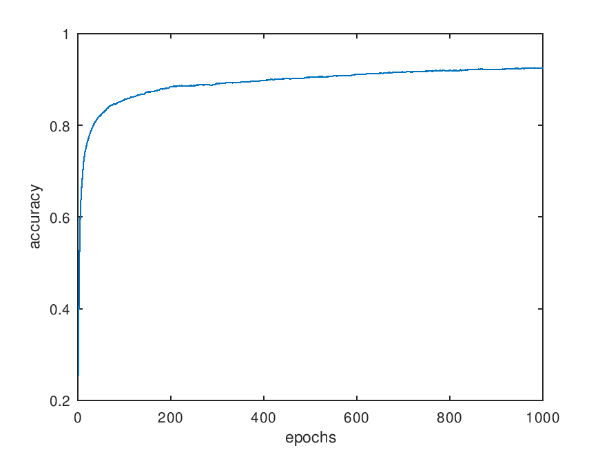
From here I wanted to see how it would do with numbers made by me, so I wrote a function to load an image and feed it to the network (I had to rotate the image since the images in the dataset were rotated 270°).
function y = load_and_feed_foward(filename)
    global A_2;
    global A_3;
    global A_4;
    global W_12;
    global B_2;
    global W_23;
    global B_3;
    global W_34;
    global B_4;

    img = imread(filename);
    img = rot90(img, 3);
    img = fliplr(img);

    image_data = reshape(img, [784 1]);
    image_data= double(image_data) ./ 255;
    imagesc(img);
    colormap(gray);
    feed_foward(image_data);
    y = find(A_4 > 0.5) - 1;
end

load_network();
disp(load_and_feed_foward("number.jpg"))
For the images I created a 28x28 grayscale canvas in GIMP and then whenever I wanted to test another drawing I just re-exported it as number.jpg
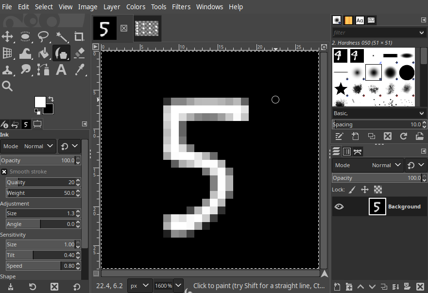
After playing with it a bit I noticed that the network classified numbers better if they were drawn below (0,5), also it has the tendency to mark 8’s as 5’s for some reason. That’s it for this post and I hope you find this topic interesting. (Get the tuned weights and biases here).
